Tagged Curriculum

0

Constructing an Introductory Science Curriculum with Text Analysis and a Path-Minimizing Heuristic Algorithm


An interdisciplinary curricular sequence was automatically generated using term-frequency–inverse-document-frequency metric and statistical analysis on a corpus of science textbooks.

Introduction

A complex body of knowledge, such as science, is composed of various concepts and ideas that overlap and interconnect with one another. For example, in the discipline of physics, the concept of energy may be used to explain the motion of an object, whereas in chemistry, the energy concept may be used to explain the release of heat during a chemical reaction. In biology, the same concept may be used to illuminate the metabolic process within a cell. Therefore, the role of a teacher is to provide a thoughtful, well-designed curriculum, or a topical trajectory through many pieces of information, and help students to integrate different concepts toward a deep understanding of a topic.

A science textbook, with its sequence of chapters and sections, is an example of a carefully-designed trajectory through topics. While such reference sequences developed by subject experts are highly valuable, different topical trajectories can also be worthwhile and perhaps more effective for different teachers or students. Students may benefit from a different entry point to a topic based on their interest or background knowledge. For example, introductory physics may be taught in different sequences, based on whether a student is majoring in physics, chemistry, or biology. Different curricular sequences would highlight different connections between concepts and generate diverse insights about a topic.

We developed a method for producing topical sequences through a corpus of science textbooks, based on text analysis and path-minimizing heuristic algorithms. This method could be useful for students or teachers of introductory collegiate science courses, in which wide-ranging topics are introduced to a group of students whose interests and backgrounds are similarly wide-ranging. A teacher may use it to develop a lesson plan that explores connections between different topics and disciplines. A biology student who knows about the membrane potential of a cell from a biology course may benefit from reading about the concept of electrical potential from a physics textbook. Conversely, a physics student may reinforce the concept of electricity by learning about electrical phenomena from a biology textbook.

Finding informative terms

The texts from college-level introductory physics, chemistry, and biology textbooks from OpenStax (OpenStax College) were collected in plain text, ignoring special characters or mathematical symbols. Each section of the textbook is referred to as a “document” and is the smallest unit of data. The collection of these documents is referred to as a “corpus.” The punctuation marks and a set of common, uninformative words (such as “the”, “and”, or “a”) were removed, and the remaining words were transformed into their rudimentary forms or word stems, by the removal of suffixes like “-s” or “-ing.” For example, after stemming, “force”, “forces”, and “forced” are transformed into the same lexicon, “forc”. After a series of these preprocessing steps, each document was reduced into a collection of stemmed terms. These textural operations were performed with Python’s Natural Language ToolKit (NLTK) module (Bird, Loper and Klein, 2009).

Then, the term frequency-inverse document frequency (tf-idf) metric (Robertson and Spärck Jones, 1976) was calculated based on the frequency of each term within all documents in the corpus, according to the following formula:

tf-idf(t,d) = tf(t,d) x idf(t) = tf(t,d) x ( log( (1+N)/(1+df(t)) ) + 1 )

where tf(t,d) denotes the number of occurrences of each term (t) in each document (d), df(t) denotes the number of documents containing a particular term (t), and N is the total number of documents. The addition of 1 within the log function is to avoid division by zero or log of zero operation.

This metric quantifies the significance or the level of informativeness of a term within a corpus of documents. Low tf-idf value indicates that a term is not used often and/or it is a very generic term that appears throughout the entire corpus, so this term is not informative. High tf-idf value indicates that a term is used quite extensively in a certain document but not too often elsewhere within the corpus, so this term is likely an informative keyword for the document.

The following table shows a few examples of high tf-idf terms within a particular document from the textbook corpus. There is a reasonable correspondence between the topic of each document and these terms in their stemmed forms. A student or a teacher may use such a list to quickly identify important vocabularies of concepts within the documents.

Section number and title

(source: PHYS/CHEM/BIOL textbooks)
Top 5 terms with large tf-idf values
PHYS 32.3 

Therapeutic use of ionizing radiation
cancer, radia, patient, tissu, ray
CHEM 6.2 

Potential, kinetic, free, and activation energy
energi, reaction, chemic, free, releas
BIOL 39.2 

Gas exchange across respiratory surfaces
volum, pressur, air, mm, oxygen
Table 1. Examples of high tf-idf terms associated with a section from Physics, Chemistry, or Biology textbook from OpenStax.

The following table lists the top hundred informative terms, ranked by their average tf-idf values within physics, chemistry, and biology textbooks as well as the entire combined corpus. For example, in physics, “force” and “energy” are highly informative; in chemistry, “atom” and “electron”; and in biology, “cell” and “plant.” They represent keywords from three major branches of science.

Corpus Terms with highest tf-idf values
Physics forc, energi, charg, wave, field, magnet, veloc, light, current, use, mass, motion, ray, object, electron, electr, two, direct, heat, one, point, temperatur, pressur, voltag, figur, momentum, acceler, time, particl, atom, speed, shown, water, imag, system, frequenc, show, resist, 10, radiat, vector, law, angl, wavelength, work, fluid, move, distanc, transfer, power, earth, sound, rotat, angular, chang, line, relat, calcul, produc, air, flow, posit, physic, circuit, kg, observ, exampl, equat, measur, given, nuclear, potenti, wire, surfac, zero, molecul, number, photon, differ, also, kinet, conserv, see, equal, valu, displac, 100, decay, first, find, part, right, length, small, exert, bodi, constant, reflect, per, weight
Chemistry
 atom, bond, reaction, label, electron, aq, energi, acid, figur, two, water, solut, molecul, ion, use, subscript, carbon, right, compound, metal, contain, mass, rate, form, structur, one, 10, orbit, pressur, concentr, arrow, group, gas, temperatur, element, show, oxid, equilibrium, chemic, sphere, number, point, solid, shown, left, liquid, cell, exampl, chang, hydrogen, superscript, oxygen, line, process, equat, heat, particl, volum, red, substanc, negat, mol, pair, diagram, reactant, tube, charg, amount, first, three, sign, law, imag, valu, unit, work, properti, ionic, chapter, calcul, second, axi, column, blue, increas, product, spontan, formula, molecular, measur, singl, solubl, constant, follow, base, oh, credit, green, relat, modif
Biology cell, plant, speci, figur, organ, protein, energi, dna, anim, gene, water, form, bodi, molecul, blood, system, show, use, popul, two, one, chromosom, call, membran, human, work, acid, hormon, produc, credit, carbon, also, differ, tissu, modif, structur, develop, group, reproduct, prokaryot, may, process, cycl, diseas, food, bind, mani, live, photo, tree, flower, life, bacteria, genet, includ, egg, function, part, environ, bone, fungi, receptor, exampl, oxygen, reaction, caus, virus, rna, signal, root, eukaryot, infect, activ, transcript, releas, type, light, result, chang, occur, contain, scientist, glucos, seed, individu, male, sequenc, enzym, atp, genom, like, fish, increas, respons, muscl, growth, electron, femal, regul, fertil
Physics + Chemistry + Biology cell, energi, forc, atom, figur, use, plant, two, water, electron, one, molecul, reaction, organ, show, mass, system, speci, form, light, charg, bond, acid, protein, wave, veloc, temperatur, work, pressur, label, point, magnet, anim, field, bodi, dna, produc, gene, carbon, shown, heat, blood, structur, time, current, object, 10, chang, exampl, direct, particl, electr, call, differ, ion, ray, also, process, group, contain, right, motion, credit, human, solut, number, modif, imag, membran, mani, law, line, speed, relat, may, move, rate, air, equat, gas, increas, oxygen, calcul, arrow, part, compound, chemic, surfac, acceler, develop, left, earth, first, radiat, three, popul, food, result, subscript, frequenc
Table 2. Top 100 terms with largest average tf-idf values.

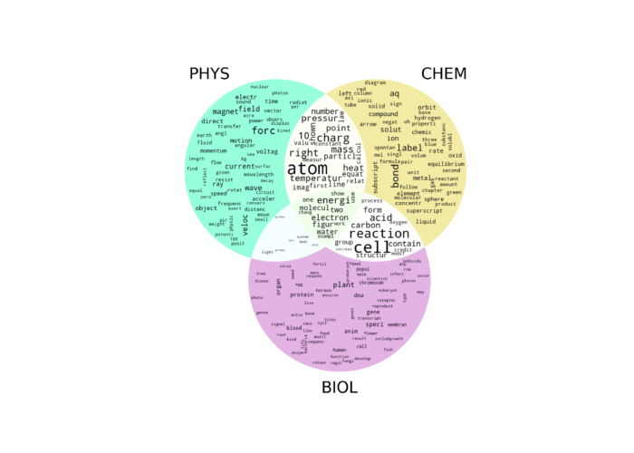
A Venn diagram of these key terms provides a way to visualize the distinctive and overlapping concepts between three major branches of science. The terms like “reaction” and “cell” are found at the intersection between biology and chemistry, and the terms like “atom” and “temperature” are at the intersection between chemistry and physics. Overlapping terms between biology and physics are fewer and tend to have lower tf-idf values. At the intersection of all three disciplines, there are such nouns as “energy”, “electron”, and “water.” The overlapping term “change” is also interesting, because scientists in all disciplines describe many important natural phenomena in terms of changes in various quantities or properties: changes in temperature, molecular structure, environments, energy, etc. The word “work” was most often used as a citation terminology in the corpus (i.e., “work by so-and-so”). Other expository terms like “example”, “figure”, “show”, and “use” are understandably used quite often across all three textbooks.

A pastel Venn diagram of terms showing their overlap in the three fields.
Figure 1. A Venn diagram of terms with high tf-idf value. The font size of each term is scaled by its maximum tf-idf value.
bar graph of tf-idf values by term and discipline
Figure 2. Bar graph of tf-idf values for each branch of science.

A breakdown of tf-idf values within physics, chemistry, and biology textbooks is shown in Figure 2 for selected key terms. The terms “cell” and “plant” have particularly high tf-idf value within biology. The terms “energy” and “force” are significant within physics, and the terms “atom” and “reaction” are significant within chemistry. These results are quite reasonable given the general focus of each discipline and indicate that tf-idf is an acceptable metric of topical significance in the corpus of science textbooks.

By considering the correlation of tf-idf values across documents, it is possible to examine which terms are closely related to one another. This examination further reveals disciplinary differences. For example, the term “energy” is highly correlated with terms like “kinetic”, “conserved”, “work”, “electron”, and “potential” within physics, while it is correlated with terms like “heat”, “acid”, “reaction”, “electron”, and “ion” within chemistry, and “reaction”, “molecule”, “cell”, “gene”, and “metabolism” within biology. The term “water” goes with “pressure”, “temperature”, “density”, “fluid”, and “heat” in physics; “liquid”, “atom”, “solution”, “electron”, and “bond” in chemistry; and “plant”, “gene”, “DNA”, “ocean”, and “cell” in biology.

An interesting term is “vector” which in physics refers to a mathematical quantity with direction and magnitude and in biology means a vehicle for delivering genetic material. Hence, in the physics textbook, it is correlated with terms like “force” (a vector quantity), “direction”, and “magnitude”, and in the biology textbook, it is correlated with “disease”, “DNA”, “transmit”, and “carry”.

Physics Chemistry Biology
Energy kinet, conserv, work, potenti, magnet heat, acid, reaction, electron, ion reaction, molecul, cell, gene, metabol
Atom electron, nucleus, molecul, forc, veloc bond, electron, reaction, structur, solut carbon, bond, molecul, electron, hydrogen
Water pressur, temperatur, fluid, densiti, heat liquid, atom, solut, electron, bond plant, gene, dna, ocean, cell
Electron atom, particl, charg, energi, wavelength atom, orbit, bond, reaction, pair reaction, atom, molecul, energi, hydrogen
Vector forc, direct, magnitud, energi, point bond, pair, electron, structur, atom diseas, human, dna, transmit, carri
Table 3. Highly correlated terms from 3 different textbook bodies. This result reveals a term has different associations and usages across different corpus.

As illustrated in Table 1, each document in a corpus can be represented by a set of tf-idf values. Section 32.3 “Therapeutic use of ionizing radiation” can be described as having high tf-idf value for the term “radia” but low tf-idf for “oxygen”. Conversely, Section 39.2 “Gas exchange across respiratory surfaces” has low tf-idf for “radia” but high tf-idf for “oxygen.” Furthermore, the pattern of tf-idf values for a fixed set of vocabulary can reveal the topical relationship between documents. For example, another document on the topic of gas would have a similar pattern of tf-idf values as Section 39.2.

Sample PHYS section graph, showing 'cancer' 'radiat' 'tissu' and 'patient' as prominent.
Figure 3. The tf-idf values from a sample section (PHYS 32.3).
Sample CHEM section graph, showing 'energi' 'reaction' 'chemic' and 'free' as prominent.
Figure 4. The tf-idf values from a sample section (CHEM 6.2).
Sample BIOL section graph, showing 'volum' 'pressur' 'air' and 'oxygen' as prominent.
Figure 5. The tf-idf values from a sample section (BIOL 39.2).

Given such quantitative representation of each document, the corpus of science textbooks can be analyzed with statistical techniques, such as Principal Component Analysis for reducing the dimensionality of the dataset into two dimensions for visualization (Jolliffe and Cadima, 2016; Pedregosa et al., 2011; Hinton and Salakhutdinov, 2006). When the entire dataset is rendered as a two-dimensional scatterplot, where each data point corresponds to an individual section and where the position of each point is determined by the principal components of tf-idf values, it is readily apparent that there are three distinct clusters, corresponding to physics, chemistry, and biology sections.

A scatter plot showing distribution of PHYS/CHEM/BIOL terms and their overlap.
Figure 6. Visualization of the corpus of science textbook, based on Principal Component Analysis of the tf-idf values. Each point in the scatter plot corresponds to individual sections.
The above scatter plot, highlighting terms 'Potential' 'Gas Exchange' and 'Therapeutic Uses.
Figure 7. The location of 3 exemple sections are shown.

Navigating through the documents

Once each document is vectorized with tf-idf values, the documents can be considered as points in a high-dimensional space or a node in a graph. The similarity, or the length of an edge, between two documents can be calculated as a pairwise distance with a Euclidean metric, for example. A total distance of a path containing multiple nodes is the sum of pairwise distances. The situation is akin to the Traveling Salesman Problem (TSP), where the objective is to minimize the traveling distance while visiting multiple cities. However, since there are many nodes (~600) in our data, it is computationally prohibitive to search for a global optimum out of ~600 factorial possible paths. Furthermore, the goal here is to explore different paths through documents and to discover interesting curricular paths, rather than to find a single best path.

A simple heuristic of hopping from the current node to the next nearest node, as long as it has not been visited before, can produce a well-determined path. Because the nearby nodes, by construction, have the similar tf-idf values, they are the documents that contain similar terms and deal with related topics. Therefore, when one navigates through such a path, there will not likely be few conceptual leaps or gaps. However, this heuristic alone is not capable of exploring diverse paths. The following stochastic process, similar to a simulated annealing algorithm (Kirkpatrick, Gelatt Jr, and Vecchi, 1983), can be added: the next nearest node may be accepted with the probability p (or the nearest node is rejected with the probability 1-p). Then, this algorithm could discover a better global trajectory, even though it contains locally less optimal path segments, as shown in the following figure.

Figure 8. Histogram of the path distances calculated using a “hard” rule (a single value) and a stochastic algorithm (100 different paths). According to the “hard” rule, the path is deterministic since the path traverses the next nearest point as long as it has not been visited before. The stochastic rule follows a similar, but not as deterministic, heuristic.

The following is an example of different paths explored by the algorithm, which start at the same document (on the topic of electric potential from the physics textbook), follow different trajectories and finish at the same document (on neural communication from the biology textbook).

An example path jumps from a start to an end across several terms on the interdisciplinary scatter plot from above.
Figure 9. An example of a path followed by the stochastic algorithm.
An example path jumps from a start to an end across many more terms than the previous path on the interdisciplinary scatter plot from above.
Figure 10. Another example of a path followed by the stochastic algorithm. It has the same starting and ending points as the previous example.

One may further analyze the paths by examining the terms with significant changes in the tf-idf values. The following figure displays the document titles of two different sample paths explored by the algorithm, along with the tf-idf values of selected terms. These terms have the largest average tf-idf values in the paths. It is noteworthy that, although these paths start and end at the same points, they involve different sets of terms and concepts. The first sample path connects the documents mostly within the physics corpus and relies heavily on the topic of electrical charge and potential. More biology documents show up in the second sample path, and some of the significant terms in those documents are energy and cell.


Figure 11. Detailed view of two different curricular paths suggested by the algorithm. The starting point was a section on electric potential energy from a physics textbook, and the ending point was a section on neural communication from a biology textbook.

Figure 12. Another detailed view of two different curricular paths suggested by the algorithm. The starting point was a section on DNA replication from a biology textbook, and the ending point was a section on Coulomb force from a physics textbook.

Discovering multidisciplinary topics

The pairwise distance between documents can be used to examine the neighborhood of a given document and the level of interdisciplinarity. A document that is close to other documents from different disciplines can be regarded as containing a highly interdisciplinary topic. For example, the neighborhood of the following documents contains other documents from biology, chemistry, and physics. More specifically, each of these documents had at least two documents from each of three textbooks among its thirteen closest neighbors. Other selection criteria of different neighborhood sizes produced similar results.

Topic Nearest Neighbors
PHYS: 32.3 Therapeutic Uses of Ionizing Radiation PHYS: 32.2 Biological Effects of Ionizing Radiation
CHEM: 21.6 Biological Effects of Radiation
PHYS: 31.1 Nuclear Radioactivity
BIOL: 16.7 Cancer and Gene Regulation
PHYS: 32.1 Medical Imaging and Diagnostics
CHEM: 21.5 Uses of Radioisotopes
PHYS: 31.2 Radiation Detection and Detectors
PHYS: 29.3 Photon Energies and the Electromagnetic Spectrum
BIOL: 17.4 Applying Genomics
BIOL: 9.3 Response to the Signal
PHYS: 14.7 Radiation
CHEM: 21.3 Radioactive Decay
PHYS: 24.3 The Electromagnetic Spectrum
BIOL: 6.2 Potential, Kinetic, Free, and Activation Energy CHEM: 5.0 Thermochemistry
PHYS: 7.6 Conservation of Energy
BIOL: 6.3 The Laws of Thermodynamics
BIOL: 6.4 ATP: Adenosine Triphosphate
BIOL: 6.0 Metabolism
BIOL: 6.1 Energy and Metabolism
PHYS: 7.0 Introduction to Work, Energy, and Energy Resources
PHYS: 32.5 Fusion
CHEM: 12.5 Collision Theory
CHEM: 5.3 Enthalpy
CHEM: 16.4 Free Energy
BIOL: 7.1 Energy in Living Systems
BIOL: 8.1 Overview of Photosynthesis
BIOL: 39.2 Gas Exchange across Respiratory Surfaces BIOL: 39.3 Breathing
CHEM: 9.3 Stoichiometry of Gaseous Substances, Mixtures, and Reactions
CHEM: 9.2 Relating Pressure, Volume, Amount, and Temperature: The Ideal Gas Law
PHYS: 11.9 Pressure in the Body
PHYS: 11.6 Gauge Pressure, Absolute Pressure, and Pressure Measurement
BIOL: 39.4 Transport of Gases in Human Bodily Fluids
PHYS: 13.3 The Ideal Gas Law
CHEM: 9.1 Gas Pressure
BIOL: 39.1 Systems of Gas Exchange
PHYS: 13.6 Humidity, Evaporation, and Boiling
PHYS: 13.5 Phase Changes
BIOL: 40.4 Blood Flow and Blood Pressure Regulation
PHYS: 11.4 Variation of Pressure with Depth in a Fluid
BIOL: 44.5 Climate and the Effects of Global Climate Change BIOL: 46.3 Biogeochemical Cycles
PHYS: 14.3 Phase Change and Latent Heat
PHYS: 13.2 Thermal Expansion of Solids and Liquids
BIOL: 44.2 Biogeography
BIOL: 27.4 The Evolutionary History of the Animal Kingdom
PHYS: 13.1 Temperature
PHYS: 14.7 Radiation
BIOL: 22.3 Prokaryotic Metabolism
CHEM: 10.4 Phase Diagrams
PHYS: 13.5 Phase Changes
CHEM: 10.3 Phase Transitions
CHEM: 18.6 Occurrence, Preparation, and Properties of Carbonates
BIOL: 8.3 Using Light Energy to Make Organic Molecules
Table 4. Most interdisciplinary sections and their nearest neighbors.

These interdisciplinary documents deal with the topics of radioactivity, energy, breathing, and climate change. The list of neighbors hints at possible multidisciplinary science curriculum. For example, a curriculum on radiation could involve a discussion about the physical attributes of radiation (e.g., photon energy and nuclear physics) as well as about its impact on biology and medicine (e.g., radiation therapy or radioisotope imaging) and chemistry (e.g., radioisotopes). A lesson on breathing could cover the topics of respiratory organ, property of gas, and physical characterization of pressure and temperature.

Reproducible codes and step-by-step guides

The Python codes and the data of the tf-idf values are available at GitHub.

There are three Jupyter Notebooks and one master data file (OS_all_M_T_title.p). The first notebook (step1_txt2tfidf_data.ipynb) reads in a set of raw text files (individual sections of the science textbooks), calculates the tf-idf values and performs statistical analysis such as Principal Component Analysis. It also saves the calculated results with a filename OS_all_M_T_title.p. The second notebook (step2_tfidf2seq.ipynb) uses the saved tf-idf values from the previous analysis, implements the path-minimizing heuristic, and produces the sequence of sections.

The last notebook (step3_user_interface) can be run as a standalone code, as long as the data file (OS_all_M_T_title.p) is present. It allows a user to build different curricular sequences based on OpenStax textbooks, by entering various starting and ending points from drop-down menus and experimenting with other parameters in the algorithm. This notebook also creates an interactive 3D scatter plot as a standalone html file (scatter_3D.html).

Figure 13. A screenshot of a Jupyter Notebook file that can be used to generate and explore potential curricular sequences with drop-down menus for choosing different starting and ending points.
Figure 14. A screenshot of an interactive 3D scatter plot. Each color-coded point corresponds to a section from the OpenStax science textbooks (physics, chemistry, and biology in red, green, and blue, respectively). The title of the section is displayed on mouse-over.

Discussion and further considerations

Natural science is broadly and imprecisely divided into three categories: physics, chemistry, and biology. Although such categorization provides a useful framework for studying the vast world of science, it is merely a rough characterization that could unfortunately obstruct the broad applicability and interrelatedness of fundamental concepts across disciplines. It is therefore important in science education to emphasize the inter- and cross-disciplinary nature of science.

In this study, we used statistical and computational techniques to analyze college-level, introductory science textbooks. Our results show that there certainly are disciplinary distinctions between physics, chemistry, and biology textbooks, but at the same time, there are multidisciplinary topics and concepts that are shared across disciplines. Radioactivity, energy, breathing, and climate change were found to be particularly conducive to cross-disciplinary lessons. We have also introduced a heuristic algorithm for generating a sequence of reading, which may be used to develop interesting, nonlinear lesson plans that are different from the linear sequence of the original textbook. It may further be used to augment the traditional curriculum and expand the curricular scope to include other disciplines. The above visualizations of science textbooks could provide students with a multidisciplinary perspective, too.

The codes for reproducing our results are made available on GitHub, and these codes may be adapted to analyze texts from other disciplines, such as social sciences and humanities. Similar approaches may be further applied to legal or healthcare documents (Hobson, 2019), while it should also be recognized that there are biases in data and limitations in algorithms (O’Neal, 2016). For example, if a certain topic is either under- or over-emphasized in the corpus of texts, the results will inherit similar biases. Our simple heuristic algorithm has the advantage of being simple and interpretable, but, because of its simplicity, its outputs are not always usable. Many of the paths that are suggested by the algorithm may not be viable as a curricular sequence, so they should be inspected by an experienced instructor before being deployed to a student body.

Bibliography

Bird, Steven, Ewan Klein, and Edward Loper. 2009. Natural Language Processing with Python. Sebastopol, California: O’Reilly. 


Hinton, Geoffrey E., and Ruslan R. Salakhutdinov. 2006. “Reducing the Dimensionality of Data with Neural Networks.” Science 313, no. 5786 (July 28): 504–7. https://doi.org/10.1126/science.1127647. 


Hodson, Richard. 2019. “Digital Health.” Nature S97, 573, no. 7775 (September 25). https://doi.org/10.1038/d41586-019-02869-x. 


Jolliffe, Ian T., and Jorge Cadima. 2016. “Principal Component Analysis: a Review and Recent Developments.” Philosophical Transactions of the Royal Society A: Mathematical, Physical and Engineering Sciences 374, no. 2065 (April 13). https://doi.org/10.1098/rsta.2015.0202. 


Kirkpatrick, Scott, Charles Daniel Gelatt, Jr., and Mario P. Vecchi. 1983. “Optimization by Simulated Annealing.” Science 220, no. 4598 (May 13): 671–80. https://doi.org/10.1126/science.220.4598.671. 


O’Neil, Cathy. 2016. Weapons of Math Destruction: How Big Data Increases Inequality and Threatens Democracy. New York: Crown Publishing.


OpenStax College. 2018. Biology 2e. Accessed June, 2019. https://openstax.org/details/books/biology-2e.


OpenStax College. 2018. Chemistry 2e. Accessed June, 2019. https://openstax.org/details/books/chemistry-2e.


OpenStax College. 2018. College Physics. Accessed June, 2019. https://openstax.org/details/books/college-physics.


Pedregosa, Fabrice, et al. 2011. “Scikit-learn: Machine Learning in Python.” Journal of Machine Learning Research 12: 2825–2830.


Robertson, Stephen. E., and Karen Sparck Jones. 1976. “Relevance Weighting of Search Terms.” Journal of the American Society for Information Science 27, no. 3: 129–46. https://doi.org/10.1002/asi.4630270302.

Acknowledgments

This project was supported by Drew University’s Digital Humanities research grant from Andrew W. Mellon Foundation.
About the Authors

Gabriel Dutra is studying Computer Science at Drew University. Dutra conducted statistical analysis of text data and developed the path-minimizing algorithm.

Ji Hoon Kim is pursuing a dual degree of Physics B.A. from Drew University and Applied Physics B.S. from Columbia University. Kim conducted the pilot study using the physics textbook.

Peiyu Guo graduated from Drew University with a B.A. in Computer Science. Guo collected data and conducted statistical analysis.

Kayla Rockhill is studying Physics and Mathematics at Drew University. Rockhill collected data.

Minjoon Kouh is an associate professor of Physics and Neuroscience at Drew University. Kouh designed and supervised the overall analysis and wrote the paper. He is the corresponding author.

and of a student in Cleveland Museum of Natural History Archives
0

Branching Out: Using Historical Records to Connect with the Environment

Abstract

What started out as an effort to digitize a small collection (two and a half linear feet) of archival material mushroomed into several interconnected projects, described here, that demonstrate the value of accessibility of historical records in the natural sciences. Funding from the National Historical Publications and Records Commission enabled the Cleveland Museum of Natural History to collaborate with Baldwin Wallace University to create an accessible online repository of original material from Cleveland naturalist A.B. Williams, and to design a curriculum for teaching with those primary sources in middle and high school classrooms. Graduate students at the University of Akron were instrumental in developing lesson plans, field trip protocols, and even a unique game from the digitized resources to facilitate learning about the different types of trees in the A.B. Williams Memorial Woods. Further collaborations followed, creating opportunities for undergraduate students at two area universities (University of Akron and Baldwin Wallace) to use the digitized data within the historical records to create georeferenced maps and to conduct a re-survey of the forest. This paper highlights how the digitization of archival materials allows for the development of numerous types of educational and research resources, with three products as proofs of concept.

Introduction: Teaching with Historical Records in the Natural Sciences

In the sciences, primary sources can be defined as records of observations in the natural world. Teaching with primary sources is an integral part of inquiry-based learning, and both archivists and educators have embraced opportunities to use archival materials in the classroom. Allowing students to use the raw material of scholarship has the potential to reap benefits. Students learn to consider different perspectives and to think critically (Hendry 2007). Students might also feel more invested in their research when they get to see original sources (Tally and Goldenberg 2005). By working with primary sources in the sciences, students can develop their own skills of observation and analysis (Austin and Thompson 2015). The Discover – Explore – Connect project was developed to introduce middle and high school students to different types of historical records in the natural sciences, such as field notes, maps, and photographs. By engaging with these primary sources, the project aims to teach and enforce the skills of observation and analysis in both the classroom and outdoors. The project demonstrates how both educational and research tools can be developed and implemented when archival materials are made accessible through digitization.
In July 2016, the Archives of the Cleveland Museum of Natural History (CMNH) received a two-year grant from the National Historical Publications and Records Commission (NHPRC). The project, titled Discover – Explore – Connect: Engaging with the Environment through Historical Records in the Natural Sciences, was part of the NHPRC’s Literacy and Engagement with Historical Records program. The funding allowed the CMNH Archives to digitize 2.5 linear feet of records relating to Arthur B. Williams, a naturalist and educator who shaped outdoor education in the Cleveland area in the 1930’s – 1950’s. Digitization not only allows access to the irreplaceable primary sources, but does so in a way that allows preservation of the original documents and materials. The material was digitized by work-study students at Baldwin Wallace University, under the supervision of the University Archivist. The students who digitized the material learned how to handle fragile documents, use scanning equipment, and assign metadata to the finished electronic documents.

With the rich resources within the A.B. Williams archive digitized, teachers, students, researchers, and citizen scientists can access and use the material to glean valuable information about the natural world around them. Several interconnected projects have been developed that draw from the A.B. Williams Archive: a curriculum that contains both classroom and outdoor experiences, including a game; GIS applications; and a re-survey of the forest that allows for comparison with the historical data.

Results: Projects Derived from Digitized Materials

Lesson plans for ecological literacy

The goal of the Discover – Explore – Connect curriculum is to teach middle school and high school students the skills necessary to study the natural world around them. Through a series of lessons, students learn orienteering, species identification, mapping, taking field notes, and collecting data, with A.B. Williams as their guide. The curriculum is divided into three major sections: Skills Development and Game-Based Learning; Field Trip to A.B. Williams Memorial Woods; and the Land Ethic.

The lesson plans in the Skills Development section introduce students to primary sources and teach them how to identify and analyze different types of primary sources, such as maps, photographs, and written documents. Students also learn how to interpret and use different types of information that can be found in scientific documents, such as charts, data tables, maps, graphs, and diagrams. Additional lesson plans guide students in making observations, keeping field notes, finding their way around a map, and recording observations on a map. Subsequent lessons help students build skills in identifying different species of wildflowers, birds, and trees.

A unique addition to the curriculum is a game that was developed as an orientation for field trips to the A.B. Williams Memorial Woods in the North Chagrin Reservation of the Cleveland Metroparks. Well-designed games have been shown to facilitate engagement with learning (Dickey 2005; Abdul Jabbar and Felicia 2015) and improve meaning-making for the players (Ermi and Mayra 2005). The game was designed to deliver three main learning outcomes: familiarize students with the layout of the A.B. Williams Memorial Woods; provide a practical tutorial in using dichotomous keys to identify wildlife; and prepare students to survey plant and animals communities in the forest. By simulating the types of activities that will take place on their visit to the forest, students should be better prepared and focused during the field trip (Falk and Dierking 2000).

For the game’s design and construction, the A.B. Williams Memorial Woods was split into five regions based on different forest communities: Beech-Maple Association; Northwest Forest; Southeast Forest; Spurs and Ravines; and Swamp Forest (Figure 1).

A map of the A.B. Williams Memorial Woods. It is divided into five color-coded regions: Northwest Forest; Spurs and Ravines; Southeast Forest; Beech-Maple Association; Swamp Forest.

Figure 1. Game map showing the different regions of the A.B. Williams Memorial Woods in the North Chagrin Reservation of the Cleveland Metroparks

Using A.B. Williams’ historical survey data of tree distributions, decks of cards were constructed for each of these regions. Each deck contains between 17 and 39 cards. Individual tree species for each region are depicted on the cards using illustrations of leaves that were drawn by A.B. Williams and are part of the digitized collection; drawings of twigs and buds were created by the project’s graphic designer to provide additional information to aid species identification. Each card provides enough information for the tree species to be identified using the provided dichotomous key or a field guide, along with a symbol to allow for easy sorting of cards based on region, and a number value to indicate how many individual trees that card represents (Figure 2).

An example of card used in the tree identification game. It depicts the leaf and stem pattern, the forest community in which it is found, and the number of individual trees the card represents.

Figure 2. Example of card showing a single species of tree to be identified

For each deck, the number of cards depicting the same tree species is based upon the proportionate number of those trees surveyed in that region by Williams in the 1930’s (Williams 1936). To keep the decks at workable sizes while allowing for representation in the deck of all the tree species in each region, the ratio of number of cards to total count of corresponding tree species is arranged upon a log scale, which results in the number of cards per species corresponding roughly with order of magnitude rather than actual counts. Accompanying these decks are a specially constructed dichotomous key (Figure 3) and data collection sheets for student groups to record distribution data (multiple cards of the same species have different numbers to simulate the actual counting activity). Instructors also have an answer and scoring sheet that allows them to track student success rates and completion times, and to check on each group’s work.

A dichotomous key for the trees found in the A.B. Williams Memorial Woods. It features 17 questions about a tree’s characteristics, each with two answers. Each answer leads to another question, which then points to the tree’s identity by the end of the questions.

Figure 3. Dichotomous key to be used for identifying trees in the A.B. Williams Memorial Woods

Gameplay requires students to work together in teams to effectively and efficiently identify the trees in each region. The game can be played while sitting at a desk, but we encourage teachers to set up the classroom as the forest and have students move around from community to community. The instructor serves as a scorekeeper to track both accuracy and speed, and each student group competes to be best at identifying and surveying tree species. As players progress through surveying each region’s deck, they will grow more proficient in using the dichotomous key to identify trees, and they will acquire information on the distributions of individual tree species throughout the A.B. Williams Memorial Woods.

Future work can not only further develop this game, but also expand upon it to include modules that examine wildflowers and songbirds, using resources made available through the digitized A.B. Williams archival material. This game is designed in such a way that it can easily be adapted to any location that has robust biological survey data, with limited adjustment to its design. The game is currently being developed to work as a standalone boxed experience that can be played like a traditional board/card game as opposed to a classroom activity.

The Discover – Explore – Connect curriculum was introduced at a teacher workshop held at CMNH in February 2018. The 18 teachers who attended the workshop included classroom teachers, homeschool parents, university/college educators, and informal science educators (i.e., museum docents, library media specialists, park naturalists). Educators worked through several lessons and played a test version of the A.B. Williams Forest Community Challenge Game. We received valuable feedback on the game and the curriculum, and this input will help as we continue to develop both for future use.

Following the workshop, we tested the curriculum and field trip with five classes of 10th-grade biology students from a school within the Cleveland Metropolitan School District. The teacher had attended the workshop in February and, because her school has an extended academic year, she was able to work through some of the lesson plans and schedule a field trip. Project team members visited the school at the end of May and introduced the A.B. Williams Forest Community Challenge Game to each of the five biology classes during the school day. Fifty students learned how to use the dichotomous key to identify trees featured on the game cards. While challenging at first, by the end of each class we could see that the students had made a lot of progress. The game set the stage for the June 22nd field trip to the A.B. Williams Memorial Woods. Team members planned a full day of field experiences at four different stations in the woods. The 27 students in attendance, accompanied by their teacher and three chaperones, were broken up into four groups. Each group was led by a member of the project team as they cycled through all four stations and completed the activities, which included counting and measuring trees within a designated area, honing observation skills while focusing on sounds, and learning about the Civilian Conservation Corps’ efforts to build a shelter in the woods in 1933.

The field trip was a rewarding experience for everyone. While guiding a group into the forest, the leader held up a large leaf that had been found on the ground. One of the students immediately noticed its shape and started to identify it based on the dichotomous key used during the A.B. Williams Forest Community Challenge game in class. Following the field trip, the teacher solicited feedback from her students. One of the students said, “The field trip was very breathtaking…A.B. Williams – I feel like I was walking on his path [and] you saw his nature as it was…I feel like what he did was awesome.”

Our hope is that the Discover – Explore – Connect curriculum will be used in classrooms throughout the school year, so that by April or May teachers and students will be ready for at least one field trip to the A.B. Williams Memorial Woods. Lesson plans for the field trip include mapping and tallying trees and comparing those numbers with what Williams observed in those same woods 80 years ago. Once back in the classrooms, students turn to lesson plans that help them reflect on the changes that have occurred in the forest ecosystem and encourage them to examine their relationship with the natural world around them.

Where in the world…? Applying GIS technologies to historical records

The digitization of the Williams collection not only provides access to more easily view the materials, but an exciting further step is to integrate the historical maps using Geographic Information Systems (GIS). GIS is database software that allows disparate data sources to be integrated and assigned to specific coordinates on a map. This process requires that features in the maps be identified and related to a spatial reference system. The term ‘georeferencing’ is used to describe this process of adding a spatial reference system to the digital image of a historical map.

Along with visually comparing maps that have been georeferenced to the same spatial reference system, the features on the map can be depicted using points, lines, and areas. These point, line, and area features can then be graphically manipulated, incorporated with other spatial data sets, and quantitatively analyzed. For example, Williams made many maps of the trees in the North Chagrin Reservation of the Cleveland Metroparks; when georeferenced, the trees drawn on these maps can be converted to points, combined with trees from other maps, and drawn in any cartographic style.

Georeferencing the hand-drawn maps from Williams was both challenging and critical to the accuracy of any derived spatial data sets. Whatever spatial uncertainty is present in the georeferencing (there was considerable uncertainty) will be propagated through any future uses of the maps. The general strategy in georeferencing is to find features on the map that can either be located on other spatial data sets, such as aerial photography or topographic maps, or can be located in the current landscape. Whether on other imagery or in the current landscape, these identifiable locations used for georeferencing the historical maps are known as ground control points or GCPs.

Because Williams included different features on different maps but did not ever include all the features on a single map, the necessary strategy was to georeference his maps by using the best ground control points from each map. For instance, features on Williams’ maps that could not move over time, such as the foundation of the Trailside Museum in the North Chagrin Reservation, provided the best way to match features on the historical map to current features in the landscape whose coordinates we can measure with global positions systems (GPS). Because there were not enough of these more permanent features, other features such as bridges and trail intersections were also used. Since these features have a higher likelihood of having moved over the past eight decades, they introduce more uncertainty into the georeferencing process. Three authors of the paper went out into field in September of 2017 to obtain the GPS coordinates of locations/objects that were present on A.B. Williams’ various maps and could potentially be used as ground control points (Figure 4).

The image shows GIS software where a map drawn by A. B. Williams is being georeferenced using coordinates of features that are still currently visible in the landscape. These features include trails, bridges, buildings, and select trees.

Figure 4. A screenshot showing one of A.B. Williams’ hand-drawn maps matched to GPS coordinates of GCPs. The table on the top right of the image shows details on the GCPs such as latitude and longitude, as well as root mean square error (RMS).

In several GIS and Cartography courses, undergraduate and graduate students were provided with digital versions of some of Williams’ maps of trees by species and ground control points generated by the instructors. Since Williams produced no single map that contained all the features that could serve as GCPs, the students were instructed to utilize a series of exterior points on the species maps derived from the original georeferencing attempt (Figure 5).

The image shows two maps. The first map shows features, such as trails and bridges that were used as ground control points when visited by course instructors. The second map is an example of a map of individual species that students georeferenced. Coordinates for easily identifiable locations were extracted from the first map to allow students to more easily and accurately georeference the second map.

Figure 5. GPS coordinates were used by instructors to georeference an A.B. Williams map (left map above) and then four clearly identifiable locations were chosen for students to use to georeference maps of individual species such as the map of red maple.

The students then georeferenced their assigned species maps and created point representations of the individual trees. This assignment covered several core GIS methods, including georeferencing, feature creation, editing attribute tables, and spatial reference system concepts, while engaging students in the creation of new geospatial data that will be used in future coursework, research, and public displays. The use of historical data also allowed an important discussion of the value of archives in change analysis and the sources and implications of uncertainty in spatial data.

The spatial data sets of tree locations created by the students in the GIS and Cartography courses were then analyzed by students in a Spatial Analysis course. The students in this course were learning to use spatial statistical methods to identify and describe spatial patterns in large data sets. The data set of tree locations created in the earlier exercise included the species of the tree, so interspecific comparisons of clustering and dispersion were done by the students using common spatial statistics, such as average nearest neighbor, quadrat analysis, and Ripley’s K function. Several of the students in the Spatial Analysis course were also in the GIS or Cartography courses, and they were able to help explain the larger story of Williams’ work to the students who had not previously been exposed to the archive. Anecdotally, student reflections suggest that the use of historical hand-drawn maps makes the presence of spatial uncertainty more obvious than with modern digital data sources. Students were able to translate the uncertainty introduced from the data source into reasonable limitations in the interpretation of results.

While the maps that are part of the Williams archive have already proven to be pedagogically valuable, we expect to continue to develop these data sources in several ways. There are still numerous maps that need to be georeferenced and have their contents converted to spatial features. Our initial experiences in this process have been positive and instructive. As more of the maps are processed, the database available for spatial analysis will also grow. This database will be utilized by students in course assignments and individual projects. As more of the maps and spatial data are completed, students in the GIS Database Design course will be learning ways to make these databases publicly available through web mapping applications.

Once the maps have been processed and converted to features, they can be compared with the results of the re-survey efforts described in the next section of the paper. This increases the value of the data from analyzing the past to investigating how the present-day forests have changed. We expect that this highly detailed spatial database of plants and animal locations over an 80-year period in a highly urbanized and industrialized region will be valuable both for research and for communicating ecological change to the broader community.

Seeing the forest through the trees

Scientific researchers are also using the A.B. Williams archive to assess changes that have occurred over 86 years in the tree community diversity, composition, and structure of the old-growth A.B. Williams Memorial Woods. Undergraduate students, along with their professor, replicated Williams’ methods to resample trees in 58 of his plots. Such re-survey studies are valuable to the field of ecology because they provide the only direct evidence of changes over time in local species diversity and abundance (Sax and Gaines 2003; Kapfer et al. 2017). Other recent studies have used legacy data to gain insights into long-term ecological processes (Vellend et al. 2013; Perring et al. 2018), but few have been long enough to see changes in tree populations and forest communities (Müllerová et al. 2015; Šebesta et al. 2011). The Williams data provides a unique opportunity to observe changes over time in a protected old-growth forest.

In 1932, Williams (1932, 1936) counted, identified, and measured all trees ≥ 0.8-cm diameter in 44 8 × 10-m plots; counted and identified all trees at least knee high in 10 30 × 30-m plots; and counted, identified, and measured all trees at least 2 m tall in 4 15 × 15-m plots. In 2018, we relocated these plots based on the georeferencing described in the previous section and using Williams’s original tree maps, which enabled us to locate remaining individual trees. We counted, identified, and measured trees according to Williams’ methods. We plan to compare stand structure between 1932 and 2018, including stem density, basal area, and the proportions of stems in different size classes. We will compare species richness, diversity, and composition using techniques such as ordination and indicator species analysis. Finally, the observed changes will allow us to examine hypotheses about which factors, such as increased deer density or tree diseases, have driven the development of this forest. We can also assess whether tree species with certain traits have tended to increase in frequency. This study will provide rare insight into how and how much a protected old-growth forest changes over time in diversity, composition, and structure, and will suggest which ecological factors are responsible for the changes. The project provides information useful to basic ecological theory and to applied ecosystem management, including the managers of A.B. Williams Memorial Woods at Cleveland Metroparks, while providing opportunities to mentor undergraduate students in research.

Conclusion

Observations by local naturalists over a long period of time can shed light on seasonal changes. By comparing the data in these historical records with current observations and digitally captured data, scientists can investigate a number of phenomena including the impacts of climate change (Primack and Miller-Rushing 2012; Primack 2014; Ledneva et al 2004). Mining the data contained in historical scientific records has become easier than ever thanks to recent digitization efforts, such as the Smithsonian Field Book Project and Biodiversity Heritage Library, but many sources of historical observations remain hidden and unused in various repositories.

The Discover – Explore – Connect project had many moving parts with three main goals: digitize and make accessible this collection of archival material, create a curriculum for middle and high school teachers, and hold training for educators to learn how to teach using these primary sources in their classrooms and outdoors. From these goals, the project expanded its scope to include other uses for the valuable data contained within the digitized material, including a game, georeferenced maps, and a re-survey of a local forest. Two and a half linear feet of historical records can be developed and used in several different and exciting ways.

Bibliography

Abdul Jabbar, Azita Iliya, and Patrick Felicia. 2015. “Gameplay Engagement and Learning in Game-Based Learning: A Systematic Review.” Review of Educational Research 85(4): 740–779.

Austin, Hilary Mac, and Kathleen Thompson. 2015. Examining the Evidence: Seven Strategies for Teaching with Primary Source. Chicago: Maupin House Publishing.

Dickey Michele. 2005. “Engaging by Design: How Engagement Strategies in Popular Computer and Video Games Can Transform Instructional Design.” ETR&D 53(2): 67–83.

Ermi, Laura, and Frans Mäyrä. 2005. “Fundamental Components of the Gameplay Experience: Analysing Immersion.” In Proceedings of the 2005 DiGRA International Conference: Changing Views: Worlds in Play, 15–27. http://www.digra.org/wp-content/uploads/digital-library/06276.4156.pdf.

Falk, J. H., & Dierking, L. D. 2000. Learning from Museums: Visitor Experiences and the Making of Meaning. Lanham, MD: Rowman & Littlefield.

Hendry, Julia. 2007. “Primary Sources in K-12 Education: Opportunities for Archives.” American Archivist 70 (Spring/Summer): 114-29.

Kapfer, Jutta, Radim Hédl, Gerald Jurasinski, Martin Kopecky, Fride H. Schei, and John-Arvid Grytnes. 2017. “Resurveying Historical Vegetation Data—Opportunities and Challenges.” Applied Vegetation Science 20 (2): 164-171.

Ledneva, Anna, et al. 2004. “Climate Change as Reflected in a Naturalist’s Diary, Middleborough, Massachusetts.” Wilson Bulletin 116, no. 3: 224-231.

Müllerová, Jana, Radim Hédl, and Péter Szabó. 2015. “Coppice Abandonment and its Implications for Species Diversity in Forest Vegetation.”Forest Ecology and Management 343: 88-100.

Perring, Michael P., Markus Bernhardt-Römermann, Lander Baeten, Gabriele Midolo, Haben Blondeel, Leen Depauw, Dries Landuyt, et al. 2018. “Global Environmental Change Effects on Plant Community Composition Trajectories Depend upon Management Legacies.” Global Change Biology 24 (4): 1722-1740.

Primack, Richard B., and Abraham J. Miller-Rushing. 2012. “Uncovering, Collecting, and Analyzing Records to Investigate the Ecological Impacts of Climate Change: a Template from Thoreau’s Concord.” BioScience 62 (February): 170-81.

Primack, Richard B. 2014. Walden Warming: Climate Change Comes to Thoreau’s Woods. Chicago: University of Chicago Press.

Sax, Dov F. and Steven D. Gaines. 2003. “Species Diversity: From Global Decreases to Local Increases.” Trends in Ecology and Evolution 18 (11): 561-566.

Šebesta, Jan, Pavel Šamonil, Jan Lacina, Filip Oulehle, Jakub Houška, and Antonín Buček. 2011. “Acidification of Primeval Forests in the Ukraine Carpathians: Vegetation and Soil Changes over Six Decades.” Forest Ecology and Management 262 (7): 1265-1279.

Tally, Bill, and Lauren B. Goldenberg. 2005. “Fostering Historical Thinking with Digitized Primary Sources.” Journal of Research on Technology in Education 38 (1): 1-21.

Vellend, Mark, Lander Baeten, Isla H. Myers-Smith, Sarah C. Elmendorf, Robin Beauséjour, Carissa D. Brown, Pieter De Frenne, Kris Verheyen, and Sonja Wipf. 2013. “Global Meta-Analysis Reveals No Net Change in Local-Scale Plant Biodiversity over Time.” Proceedings of the National Academy of Sciences 110 (48): 19456-19459.

Williams, Arthur B. 1932. “A Preliminary Study of a Beech-Maple Climax Community.” PhD diss., Case Western Reserve University, Cleveland, Ohio.

Williams, Arthur B. 1936. “The Composition and Dynamics of a Beech-Maple Climax Community.” Ecological Monographs 6: 317-408.

Appendix: Methods

Future usability of the digitized material was maximized through the methods of processing.

  • All scans were saved as non-compressed, lossless TIFFs at 600 dpi and then stitched together to create multi-page PDFs, to allow both maximum resolution and perusal.
  • Digitizers at BW used an ATIZ BookDrive DIY cradling book scanner, complete with two mounted Canon Rebel T2i 18.0 MP digital cameras and proprietary software.
  • Individual documents were scanned on an Epson Perfection V33 flatbed scanner, and an ELMO TT-12i overhead document camera was used to digitize the most fragile documents, such as a scrapbook of cyanotype photograms from 1910-1915.
  • Once digitized and converted to PDFs, all applicable text was OCRed via Adobe Acrobat Pro DC and then uploaded to an online collection hosted by BW using OCLC CONTENTdm. Metadata was assigned using Library of Congress Authorities.

About the Authors

Thomas R. Beatman is an Integrated Biosciences Ph.D. candidate in the Biology Department at the University of Akron. His dissertation is on the theory and application of using games and gameful experiences. He uses his background in biology in the design and development of science communication toolkits to translate complex biological problems to be more understandable to the public. His primary interest is in communicating biodiversity and evolution in informal science education environments.
Shanon Donnelly is an Assistant Professor in the Department of Geosciences at the University of Akron, where he uses geospatial technologies in teaching and research. He employs tools such as geographic information systems and remote sensing in the pursuit of connecting people’s lived experiences with emergent patterns of impact and opportunity across spatial and temporal scales.
Kathryn M. Flinn is an ecologist and Associate Professor of Biology at Baldwin Wallace University in Berea, Ohio. She earned a Ph.D. in Ecology and Evolutionary Biology from Cornell University. Her recent research examines plant community change through time in northeast Ohio. With two undergraduate collaborators, she assessed changes in an old-growth forest over 86 years by resurveying A.B. Williams’s plots. The results are forthcoming in Journal of the Torrey Botanical Society.
Jeremy M. Spencer is an Assistant Professor of Instruction in the Department of Geosciences at the University of Akron. He received his Ph.D. in climatology from Kent State University, where he focused on the impact of cold weather on human mortality. Currently, his academic interests involve the communication of climatology and geography. This includes outreach to local elementary and middle schools, as well as developing course materials that promote inquiry and critical thinking in college geography and atmospheric science courses.
Ryan J. Trimbath is an Ecologist and Natural Resource Manager with broad interest in understanding and protecting nature. He received a B.S. in Wildlife and Conservation Biology from Ohio University and is a Ph.D. candidate in Biology at the University of Akron. Ryan feels lucky to have opportunities to study forests across the country from Hawaii to New Hampshire.
Wendy Wasman is the Librarian & Archivist at the Cleveland Museum of Natural History in Cleveland, Ohio, where she oversees the 50,000-volume research library, curates the rare book collection, and manages the archives and special collections. She earned a B.A. from Oberlin College and an M.L.S. from Kent State University.


Images are for demo purposes only and are properties of their respective owners. ROMA by ThunderThemes.net

Skip to toolbar
